In Galerkin method, the discretization of the governing equation is achieved through converting it into a weak formulation with a finite number of trial and test functions. The weak formulation consists of integrals defined in the simulation domain and Neumann/Robin boundaries. To calculate these integrals defined on physical domain, the general strategy, in one sentence, is to convert it into an equivalent integral define on a corresponding reference domain by coordinate transformation and integrate by numerical quadrature. To illustrate how it works, we first consider a one-dimensional case with both coordinate transformation and numerical quadrature, then extend it to higher dimensional cases.
A simple 1D example
Suppose we have a physical field $f$ defined on a line segment $[x_a,x_b]$, which is mapped from $[-1,1]$ by an affine mapping. The integral of $f$ on that segment
$$ \int_{x_a}^{x_b} f(x) \text{ d} x = \int_{-1}^{1} f(\xi) \frac{\partial x}{\partial \xi} \text{ d} \xi $$where $f(\xi)=f(x(\xi))$. The above process is called coordinate transformation, and $\partial x / \partial \xi$ is the determinant of Jacobian in 1D case, whose general form is $J_{ij} = \partial x_i / \partial \xi_j$. The integral on the rhs is calculated by numerical quadrature as,
$$ \int_{-1}^{1} f(\xi) \frac{\partial x}{\partial \xi} \text{ d} \xi = \sum_q w_q \left.\left(f\frac{\partial x}{\partial \xi}\right)\right\vert_{\xi_q} = \sum_q w_q g(\xi_q) $$Each blue cell has width $w_q$,height $g(\xi_q)$ and contains its node $\xi_q$. The map multiplies widths by $J$ and divides heights by $J$, so each cell keeps its area.
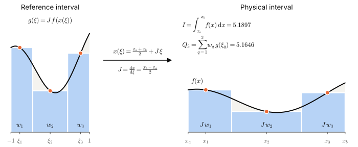
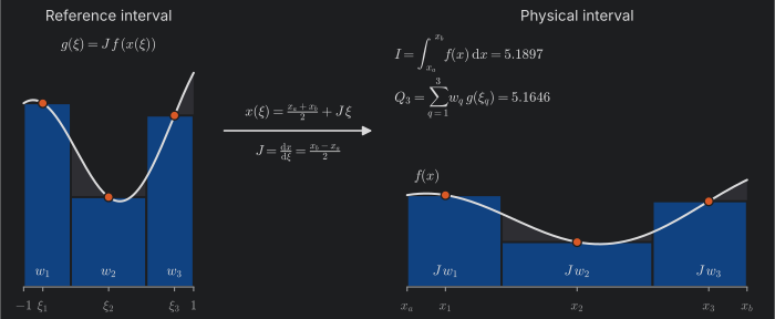
Fig. 1. Affine map from $[-1,1]$ to $[x_a,x_b]$ and the 3-point Gauss–Legendre rule as a weighted sum.
Gauss–Legendre quadrature
Then we will dive into the area of Gauss–Legendre rules, which is used for numerical quadrature with the reference interval $[-1,1]$ divided into several cells with length $w_i$. Every node lies inside its own cell. Nodes crowd toward $\pm1$ but never reach the endpoints. A $n$-point rule can integrate polynomials of degree $\le 2n-1$ exactly.
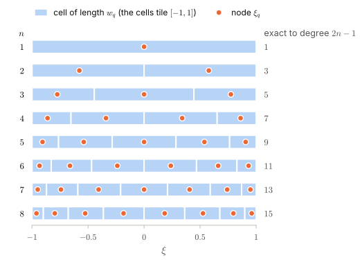
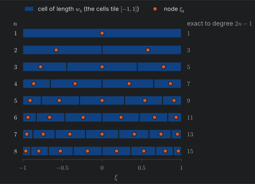
Fig. 2. Gauss–Legendre rules in $[-1,1]$ for $n=1,\dots,8$.
2D isoparametric mapping
To extend the above 1D affine mapping to 2D case, we introduce the isoparametric mapping from reference domain $\hat\Omega = [-1,1]^2$ to physical one $\Omega_e$. The green and blue lines are still straight, but on longer parallel after this mapping. Similarly, the physical domain is where the actual simulation domain is discretized, while the reference domain is where we calculate the integral in the weak formulation. Now the jacobian is a 2-by-2 matrix,
$$ \boldsymbol{J}=\dfrac{\partial(x,y)}{\partial(\xi,\eta)}=\begin{bmatrix}\partial x/\partial\xi & \partial x/\partial\eta\\ \partial y/\partial\xi & \partial y/\partial\eta\end{bmatrix} $$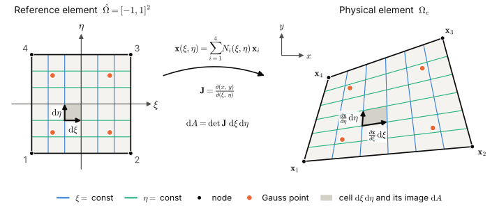
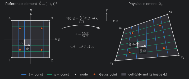
Fig. 3. Bilinear isoparametric map from the reference domain $\hat\Omega$ to a physical quadrilateral $\Omega_e$.